Details
Due date
This assignment is due on Monday, May. 13th, at 11:30 PM.
Coverage
This assignment covers the material up to Week 6, focusing on data
visualization with Matplotlib's pyplot library.
matplotlib.pyplot
This assignment involves programming with matplotlib.pyplot.
You can find all of the material needed to work with matplotlib
in Week 5/6 materials (the most useful resource will be the Matplotlib slide deck and lecture code done in class).
Do not use any other functions/modules that we haven't covered in your Part A and Part B solutions.
For example, pandas and numpy are not allowed in Part A or B, though you may see examples
in Matplotlib's documentation (which is why we provide everything you need in the lectures and posted readings).
You are more than welcome to explore these in Part C though!
What to hand in
You will be submitting 3 files to CodePost for this assignment:
mp5_parta.pymp5_partb.pymp5_partc.py(and any datasets used in this program, as well as a.pngfile of your graph(s), e.g. in the namepartc_graph.png)
Part C is a small creative component where you will choose a data set
and question of interest, and plot a graph with 1) two or more Axes or 2) a different type of plot.
You may use any dataset of interest, including lecture datasets (when we introduced csv-processing), lab datasets,
your own bottle rocket trial data CSV, planets.csv,
or any other datasets you find.
More details are provided in the Part C Overview.
Showcase: We encourage students to showcase their creations with the class! You can opt-in to the Creative Showcase (anonymous or non-anonymous) here. Don't worry about perfection/using anything beyond what we've taught; we'd like to showcase a variety of different ideas, data science questions, creativity, etc!
Supporting files
You will be finishing Part A and Part B using the provided starting code, and we have also given you a starter template for Part C:
We have also provided a single utility function used in Part B, factored out in a provided mp5_utils.py, as well as a dataset you will
be visualizing in Part B. Both of these should be located in the same directory as your solutions.
While you are not to use features we haven't covered in Part A/B, there is a small
case motivating numpy's arange function in the generate_rocket_positions function for both parts.
This function is a special version of range that has better support for non-int range
generation (recall that the built-in range function we've been using requires int values).
Since our rocket launch data is best visualized with a smoother line, we want to support float values in the
generated ranges, so you'll see this used once per file. You are not to modify it, but will want to make
sure you have numpy installed for your programs to work (and it's a good library to have
installed for later data-processing projects as well!).
To install everything you need (we recommend at this step in your reading, before starting the project), enter the following
in the bash command (similar to what you've been doing whenever using pip3, ignoring the $ prompt or whatever
your system uses):
$ pip3 install matplotlib
$ pip3 install numpy
Or:
$ python3 -m pip3 install matplotlib
$ python3 -m pip3 install numpy
Once you do this, restart VSCode just in case to make sure they are installed.
Program Overview: Plotting Bottle Rocket Launches with Matplotlib
Your tasks will be broken down into 3 Parts. In Part A, you will implement some basic functions to calculate data that is needed to plot a bottle rocket trajectory using gravity, initial velocity, and angle of launch.
Part A will fix these three experimental variables as program constants
(indicated with UPPER_CASE conventions).
We have given you most of the plotting code for this part,
which you will modify for varying trial data in Part B.
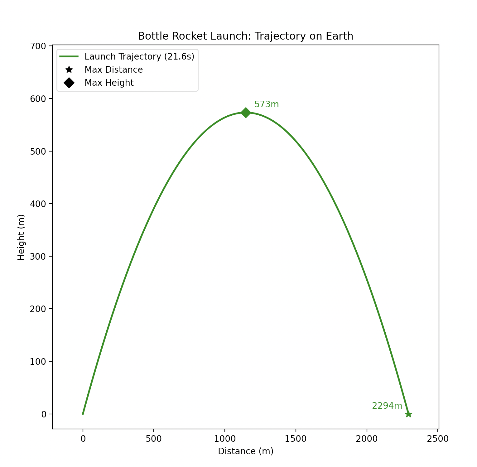
You can see a preview of what you're implementing in Part A below:
In Part B, you will take your functions from Part A and parameterize them
to replace the three data-dependent program constants.
This is an exercise of refactoring and motivating trade-offs between program constants
and parameters. Part B (and C) will also give you opportunities to practice using strategies discussed
in recent lectures, including "reverse engineering" matplotlib examples, experimentation, and
VSCode debugging.
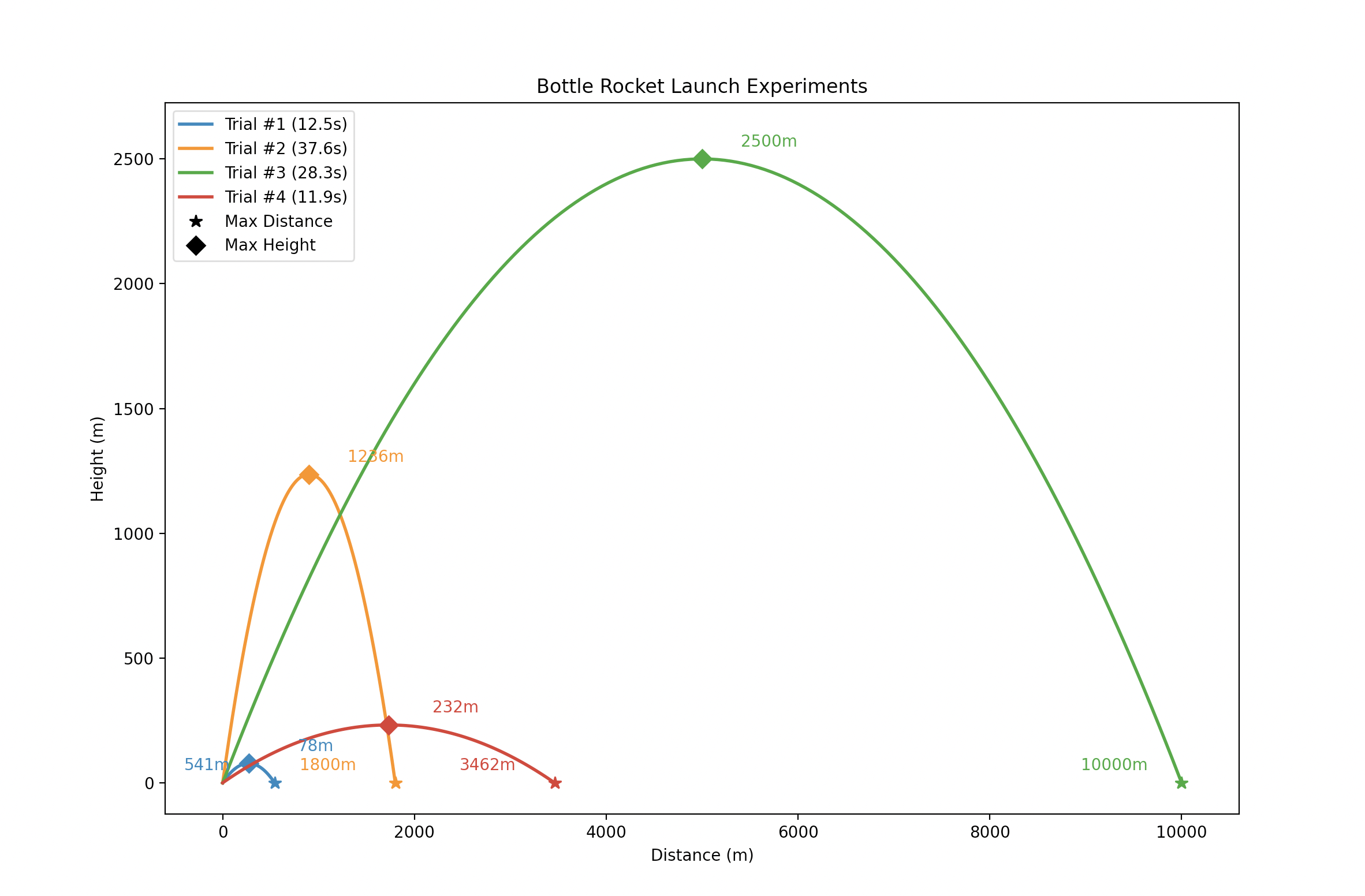
Whereas in Part A you will plot a single trajectory using the fixed program constants, in Part B you will use your parameterized functions and modified plotting code to plot data for 4 trials with different bottle rocket launch variables.
You can see a preview of what you're implementing in Part B below:
Finally, Part C will involve exploring another data visualization approach,
either 1) plotting data on two or more plots (Axes) instead of one
or 2) using a different type of plot (bar, histogram, pie, heatmap, etc.).
This part is introduced as an opportunity to apply what you've been learning in
a creative way, starting with a data set of interest and a question you want to ask about the data that can be visualized using Matplotlib.
To summarize, all the plots you will be seeing should belong to a single Figure (per program) which has:
- Part A: 1
Axes, 1 Line with 2 Points - Part B: 1
Axes, 4 Lines (2 Points per Line) - Part C: Option 1 (two or more
Axes, at least one plot each) or Option 2: Using different plot types (bar, histogram, scatterplot, pie, etc.)
Part A: A Simple Bottle Rocket Launch Plot
Summary
We have given you starter code for Part A in mp5_parta.py
you will note three program constants at the top of the program:
GRAVITY = 9.81          # m/s^2
ANGLE_OF_LAUNCH = 45    # in degrees from horizon
INITIAL_VELOCITY = 150  # m/s, fixing the initial velocity v0
You will also see some constants that will not be involved in parameterization; these will be unchanged, but demonstrate good use of constants for program-wide settings, especially when doing graphics programming.
# Offsets for point labels (e.g. max height and landing point annotations)
X_LABEL_OFFSET = 150
Y_LABEL_OFFSET = 10

# Default marker size for plotted points
MARKER_SIZE = 8
LINE_WIDTH = 2
Note that the two offsets could alternatively be implemented as factors (e.g. 5% to generalize the label positioning based on axis scales, but to make it easier to test without floating point subtleties, you will use these constant offsets for Parts A and B (you can choose your own implementation in Part C).
Note that we could also parameterize launch starting positions, but we will not add that support in MP5. You can assume that every launch in Part A/B starts at the position (0, 0), which we've noted in the starter code for you (this will also simplify edge cases with quadratic equations that could otherwise have two solutions).
Final reminders for getting started:
- Make sure you think carefully about the DRY principle in this assignment! We are looking for you to not only learn how to use Matplotlib, but also to (continue to) think about how to use functions you've already implemented to avoid redundancy, as well as being able to identify the trade-offs between Part A and Part B.
- Most of the solutions are fairly short, especially since you are finishing partially-completed solutions. Most of the time spent should be on understanding the problem, utilizing the VSCode debugger when you're stuck on common bugs (usually relating to data types of variables at each step), and referring to course materials (e.g. the lecture slides and notes) to piece things together.
- Use the program constants in Part A as given! Some will then be replaced in Part B as function parameters.
- Don't forget to refer to Part A when working through Part B.
- Test iteratively! Once you finish a function, test it in the interpreter without plotting to make sure you get the expected results for valid arguments. Make sure the data types match the spec!
- Don't worry about the
np.arangefunction more than commented; you are not using numpy anywhere else in Parts A/B. - Have fun!
1. calculate_velocity
[10]
First, you'll write a function called calculate_velocity which takes no arguments, but uses the program constants
to calculate the vx and vy velocities of the rocket based on an initial velocity,
a launch angle (e.g. 45 for 45 degrees from the horizon).
The function should return a tuple representing the velocity vector of vxi and vyi float values,
which represent the velocities in the same units as INITIAL_VELOCITY.
To calculate velocity, remember from your physics fundamentals to
use cos (for x velocity) and sin (for y velocity). We have already
imported the math module for you in the starter code for these functions.
Since the ANGLE_OF_LAUNCH
is in degrees (this makes it easier for users to specify angles),
you'll need to convert to radians. You can convert degrees to radians easily with
math.radians(<degrees>).
math.radians(0)   # 0.0
math.radians(360) # 6.283... (2pi)
math.radians(90)  # 1.5707...(pi/2)
Using the provided program constants, a call to calculate_velocity() should return the tuple (106.06601717798213, 106.06601717798212) (what happens when you change the INITIAL_VELOCITY and ANGLE_OF_LAUNCH constants?).
For reference, our solution is 5-6 lines ignoring comments. Make sure to use variables to avoid recomputation!
2. calculate_position
[5]
Next, you'll use your calculate_velocity function to implement calculate_position. This function
takes a single parameter dt representing the time elapsed, and returns the (x, y) position (a tuple)
of the rocket at dt.
We have given you the launch starting position, which we will fix at (0, 0) to keep things simple.
Here are some example calls and the expected results for the provided program constants constants (again, these constants should be used in this function):
>>> from mp5_parta import calculate_position
>>> calculate_position(0)
(0.0, 0.0) # Remember that this is the evaluation, not any unspecified print output
>>> calculate_position(1)
(106.06601717798213, 101.16101717798212)
>>> calculate_position(10)
(1060.6601717798212, 570.1601717798212)
>>> calculate_position(21.62406058674457)
(2293.577981651376, 0.0)
If you change ANGLE_OF_LAUNCH to 90,
observe the difference (again, remember to change it back to the provided constants in your solution):
>>> from mp5_parta import calculate_position # after experimenting with change
>>> calculate_position(0)
(0.0, 0.0)
>>> calculate_position(10)
(9.184850993605149e-14, 1009.5)
If you then change back ANGLE_OF_LAUNCH to 45, and change INITIAL_VELOCITY from 150 to 10, note the difference:
>>> from mp5_parta import calculate_position # after experimenting with change
>>> calculate_position(0)
(0.0, 0.0)
>>> calculate_position(10)
(70.71067811865476, -419.78932188134524)
We can observe that at 10 seconds into the launch, the y position
would be below ground level (why?). What do you think predict will happen if you change the GRAVITY constant?
Already, we can see some of the limitations with program constants in this case. When we're exploring the results of changing different variables, supporting parameters for these will be very useful! But for Part A, our goal is to just get started plotting a simple example with these variables fixed.
For reference, our solution is 5-6 lines ignoring comments.
3. flight_time
[5]
One of the important measurements of a bottle rocket launch is the total time of flight (sometimes referred to TOF).
Finish this function to compute the total flight time (which will be in the same units as INITIAL_VELOCITY and GRAVITY).
Again, we are assuming the default starting position of (0, 0).
To calculate the total flight time, you'll need to figure out the initial y velocity (use your calculate_velocity function)
and the GRAVITY constant. Remember that velocities and gravity in this program have compatible units,
both involving seconds. Refer to your physics classwork to determine the total flight time from this information.
The time should be returned as a float. For the current program constants, you should expect a call to flight_time() to be 21.62406058674457.
For reference, our solution is 2-3 lines of code and the only constant it references directly is GRAVITY.
4. generate_rocket_positions and 5. plot_labels
Next, you'll add specified comments to A.4. and A.5 and modify a single line of code in A.6. We recommend you do A.6 before you attempt A.5 so that your VSCode debugger works properly. The rest of the functions are given to you in Part A, and you are expected to spend 3-5 minutes understanding what they do in the full program execution (we encourage you to use the VSCode debugger). You will modify some of these in Part B using your parameterized functions.
Here's a brief summary of A.4. and A.5. to get you started:
-
generate_rocket_positionsuses the functions you've implemented so far to generate the data for your launch given a total flight time. -
plot_labelsfactors out the plotting of the 2 points of interest for each launch: the coordinates of the peak of the launch, and the coordinates of the landing point. This function takes a singleAxesargumentax. Remember thataxis anAxesobject generated from(fig, ax) = plt.subplots()(see the providedstartfunction) which is used to plot visualizations on a mainFigure.
For A.4. and A.5., you will demonstrate your understanding of the provided function through the following requirements (these are only required for the versions in Part A).
4. generate_rocket_positions
[10]
Write a docstring for this function that describes the behavior of the function given the single parameter, including what is returned (do not copy/paste what we wrote above). Follow the same conventions as we've shown in class, including:
- Omitting any implementation details, like loops and any local variables (including local variables that are returned, but you should specify the names of function parameter when describing them)
- Specifying the types of the parameter and return
- Any preconditions/edge cases that the function requires (you don't need to change the implementation; use your docstring to specify any preconditions)
Hint: The most important thing to make sure you understand is the relationship between
the local xs and ys variables. Are there any notes
about their lengths? Is there a relationship between xs[i] and ys[i]
in the context of a rocket launch position?
5. plot_labels
[5]
ATTEMPT THIS AFTER YOU FINISH A.6, otherwise your VSCode debugger may not work.
We've given you this docstring, but to make sure you are set up for the rest of the assignment,
you are required to add replace the 4 TODO comments in to the body of this function
with the corresponding value (as a # comment):
- The value of
dist_labelfor the Part A data - The value of
dist_label_coordsfor the Part A data - The value of
maxh_labelfor the Part A data - The value of
maxh_label_coordsfor the Part A data
This requirement is less about documentation, but more to make sure you are able to use the VSCode debugger to determine this information. At this point, we definitely expect you to know how to use the debugger, but if you run into any questions, we're happy to help.
For example, if we were to ask you to do the same thing for the code below,
we would expect the TODO replacements in the following format:
# TODO 0: Replace this line with the tuple values of (total_dist, last_y)
(total_dist, last_y) = landing_pt
...
# TODO N: Replace this line with the string value of legend_label
legend_label = f'Launch Trajectory ({tof:.1f}s)'
Replacing the TODOs as described:
# (2293.577981651376, 0.0)
(total_dist, last_y) = landing_pt
...
# 'Launch Trajectory (21.6s)'
legend_label = f'Launch Trajectory ({tof:.1f}s)'
Some notes about A.5.
This function uses the ax.annotate method to specify the
following arguments used to annotate a point with text
(in this example, no arrow is used but the documentation includes examples using arrows).
You can find more about the arguments from the official Matplotlib documentation if you're curious.
Here's a quick summary of the annotation arguments we're using:
- The
textis the label. - The
xykeyword argument is the (x, y) tuple associated with the annotation. - The
xytextkeyword argument is the (xt, yt) tuple associated with the text of the annotated point. Note that the two offset constants are used to avoid overlapping the text with the annotated point. - The
colorof the annotation is the same as the plotted point. - The
horizontalalignmentkeyword is centered so that we can standardize placement of labels.
In addition to plotting the point and its annotation, you'll see ax.set_xlim and ax.set_ylim to set the
x and y axis ranges, respectively. Why do we set these? If you experiment commenting out these lines, you'll notice that
the landing point marker will be cropped off at y = 0, and the annotation label above the
highest point will be cropped off above the upper-bounds of the plot.
6. plot_launch
[5]
The last step in Part A is to add a single line in plot_launch to plot the
launch trajectory!
This is the main function for plotting the launch given the three program constants (which you will parameterize in Part B) and plotting configurations.
Use the comments as well as an understanding of your functions so far to familiarize yourself with the plotting code.
Replace the TODO in this function to plot the
line for the trajectory, following the instructions in the starter code.
The replaced comment/code should only be two lines (a single statement broken into
2 lines to keep the line under 80 characters). Now that you have completed the function,
you can go back and fill in the TODO comments from A.5 using the VSCode debugger.
The Rest (Provided)
The rest of the code is given to you; there is nothing for you to add (code or documentation-wise). We've summarized these functions briefly for you.
configure_plot
As mentioned in lecture, our primary source of interaction with Matplotlib is the Axes object(s) returned from plt.subplots(). When
you work on data visualization programs, there is more than just plotting your data, and usually there are configurations you will want to override to improve the quality/interpretability of your visualization(s).
This function factors out the configurations specific to the the Figure and Axes and unrelated to the actual lines/points. You'll note that we plot two black points to add to the legend; we use black ('k') to generalize the legend markers for larger visualizations
like Part B so we don't have so many legend items.
You'll also see the x and y limits updated here to give some padding to the Figure for the points and annotations to fit. How would one choose these values? Well, in practice you'll want to be considerate of the likelihood of your x and y axis ranges changing
(e.g. and an offset of 100 looks much different when the upper-bound is 50 vs. 1000). With more experience, one would be encouraged to use relative offsets with percentages, but for the scope of this assignment we just give you constant values.
You are welcome to keep these as-is or be a bit more clever in Part C.
start
Finally, we see the starting point for everything working together! Just like in previous assignments/labs/lecture code, having a short start function is good practice to have good program decomposition. This is where we create the Figure and Axes, and pass ax to any functions that need it (fig isn't used in any other functions, so it shouldn't be passed anywhere).
Part B: Parameterizing Launch Variables
1. calculate_velocity
[5]
First, you'll modify calculate_velocity to take two arguments (vi and launch_angle)
to remove the dependency on the respective program constants.
This parameterization will allow us to generalize the functions
to plot different graphs in Part B to compare the results of
changing different experimental variables.
As with Exercise A.1., the function should still return a tuple representing the velocity
vectors vx and vy, and should treat the parameters the same (e.g. launch_angle
is still expected to be in degrees, vi is expected to be compatible with
gravity units).
For reference, your solution should be the same length as A.1 and should
return the same result when called with INITIAL_VELOCITY, ANGLE_OF_LAUNCH.
Here are some example calls and expected results of your parameterized implementation:
>>> import mp5_parta # avoid naming conflict
>>> mp5_parta.calculate_velocity() # non-parameterized version
(106.06601717798213, 106.06601717798212)
>>> from mp5_partb import calculate_velocity
>>> INITIAL_VELOCITY = 150 # m/s, sanity check with Part A values
>>> ANGLE_OF_LAUNCH = 45   # in degrees from horizon
>>> calculate_velocity(INITIAL_VELOCITY, ANGLE_OF_LAUNCH)
(106.06601717798213, 106.06601717798212)
>>> calculate_velocity(150, 90)
(9.184850993605149e-15, 150.0)
>>> calculate_velocity(150, 60)
(75.00000000000001, 129.9038105676658) # floating point arithmetic isn't perfect
>>> calculate_velocity(150, 30)
(129.9038105676658, 74.99999999999999)
>>> calculate_velocity(100, 45)
(70.71067811865476, 70.71067811865474)
>>> calculate_velocity(10, 45)
(7.0710678118654755, 7.071067811865475)
>>> calculate_velocity(0, 10)
(0.0, 0.0)
>>> calculate_velocity(10, 0)
(10.0, 0.0)
2. calculate_position
[5]
Next, you'll modify calculate_position to take three additional arguments, replacing
any occurrences of global constants with the corresponding parameter values.
The initial position should still be set at (0, 0).
The following are example calls and expected returns, starting with the examples shown from Part A.2.
>>> from mp5_partb import calculate_position
>>> INITIAL_VELOCITY = 150 # m/s, sanity check with Part A values
>>> ANGLE_OF_LAUNCH = 45   # in degrees from horizon
>>> GRAVITY = 9.81         # m/s^2
>>> calculate_position(0, INITIAL_VELOCITY, ANGLE_OF_LAUNCH, GRAVITY)
(0.0, 0.0) # We haven't moved at t=0
>>> calculate_position(1, INITIAL_VELOCITY, ANGLE_OF_LAUNCH, GRAVITY)
(106.06601717798213, 101.16101717798212)
>>> calculate_position(10, INITIAL_VELOCITY, ANGLE_OF_LAUNCH, GRAVITY)
(1060.06601717798213, 570.16017)
>>> # Testing the time-of-flight from Part A
>>> calculate_position(21.62406058674457, INITIAL_VELOCITY, ANGLE_OF_LAUNCH, GRAVITY)
(2293.577981651376, 0.0)

>>> # Experimenting with some variables
>>> # Changing velocity at dt=1
>>> calculate_position(1, 100, ANGLE_OF_LAUNCH, GRAVITY)
(70.71067811865476, 65.80567811865474)
>>> calculate_position(1, 50, ANGLE_OF_LAUNCH, GRAVITY)
(35.35533905932738, 30.45033905932737)
>>> calculate_position(1, 1, ANGLE_OF_LAUNCH, GRAVITY)

(0.7071067811865476, -4.197893218813453) # what does this mean?
>>> # Changing launch angle at dt=1 (try other values of dt)
>>> calculate_position(1, INITIAL_VELOCITY, 30, GRAVITY)
(129.9038105676658, 70.09499999999998)
>>> calculate_position(1, INITIAL_VELOCITY, 60, GRAVITY)
(75.00000000000001, 124.9988105676658)
>>> calculate_position(10, INITIAL_VELOCITY, 60, GRAVITY)
(750.0000000000001, 808.538105676658)

>>> # Changing gravity constant
>>> calculate_position(1, INITIAL_VELOCITY, ANGLE_OF_LAUNCH, 1)
(106.06601717798213, 105.56601717798212)
>>> calculate_position(1, INITIAL_VELOCITY, ANGLE_OF_LAUNCH, 100)
(106.06601717798213, 56.06601717798212)
>>> calculate_position(10, INITIAL_VELOCITY, ANGLE_OF_LAUNCH, 1)
(1060.6601717798212, 1010.6601717798212)
>>> calculate_position(10, INITIAL_VELOCITY, ANGLE_OF_LAUNCH, 100)
(1060.6601717798212, -3939.339828220179) # what does this mean?
3. flight_time
[5]
Next, modify flight_time to take three additional parameters, replacing
any occurrences of global constants with the corresponding parameter values.
The launch_angle variable should be treated as degrees, just like
in Part A. Again, A.3. and B.3. should still have the same number of lines.
>>> from mp5_partb import flight_time
>>> # Testing with Part A's constant values
>>> INITIAL_VELOCITY = 150 # m/s, sanity check with Part A values
>>> ANGLE_OF_LAUNCH = 45   # in degrees from horizon
>>> GRAVITY = 9.81         # m/s^2
>>> flight_time(INITIAL_VELOCITY, ANGLE_OF_LAUNCH, GRAVITY)
21.62406058674457
>>> # A few more examples
>>> flight_time(1, ANGLE_OF_LAUNCH, GRAVITY)
0.14416040391163046
>>> flight_time(5, ANGLE_OF_LAUNCH, GRAVITY)
0.7208020195581524
>>> flight_time(500, ANGLE_OF_LAUNCH, GRAVITY)
72.08020195581523
>>> flight_time(5000, ANGLE_OF_LAUNCH, GRAVITY)
720.8020195581523
>>> flight_time(INITIAL_VELOCITY, 30, GRAVITY)
15.290519877675838
>>> flight_time(INITIAL_VELOCITY, 60, GRAVITY)
26.483957302276412
>>> flight_time(INITIAL_VELOCITY, ANGLE_OF_LAUNCH, 1)
212.13203435596424
>>> flight_time(INITIAL_VELOCITY, ANGLE_OF_LAUNCH, 50)
4.242640687119285
>>> flight_time(INITIAL_VELOCITY, ANGLE_OF_LAUNCH, 100)
2.1213203435596424
4. generate_rocket_positions
[5]
Next, you'll update generate_rocket_positions from Part A to use
your parameterized functions. This version takes three additional parameters of interest
for determining positions of a rocket during its launch. Use these
parameters appropriately to call your parameterized Part B functions.
The function should still return a single (list, list) tuple representing the information specified in Part A.
>>> from mp5_partb import flight_time, generate_rocket_positions
>>> # Testing with program constants from Part A
>>> GRAVITY = 9.81 # m/s^2
>>> ANGLE_OF_LAUNCH = 45 # in degrees from horizon
>>> INITIAL_VELOCITY = 150 # m/s LOCK THE VELOCITY
>>> from mp5_partb import flight_time
>>> # Note: there's a trade-off here between calling flight_time in generate_rocket_data
>>> # since we can compute it from the other variables, but the given
>>> # approach will be a bit more efficient/generalizable if we want to generate partial data
>>> tof = flight_time(INITIAL_VELOCITY, ANGLE_OF_LAUNCH, GRAVITY)
>>> tof
21.62406058674457
>>> xs, ys = generate_rocket_positions(INITIAL_VELOCITY, ANGLE_OF_LAUNCH, GRAVITY, tof)
>>> len(xs)
218 # based on step size in function
>>> len(ys)
218
>>> xs[0] # initial x
0.0
>>> ys[0] # initial y
0.0
>>> xs[1]
10.606601717798213
>>> ys[1]
10.557551717798214 # why is y smaller for a 45deg launch?
>>> xs[-1]
2293.577981651376 # total distance traveled
>>> ys[-1]
0.0 # back to ground
5. plot_trial_data
[10]
Finish the following TODOs in plot_trial_data to generate line graphs and max height/max distance
labels for each trial. Remove each TODO comment when you are done.
- Use your
generate_rocket_positionsto generate the x and y lists for the launch coordinates using the appropriate parameters. -
Determine the highest (x, y) point on the chart
using your
calculate_positionfunction. Remember that the peak of the trajectory (without resistance/etc.) is exactly at the middle of the launch time. - Plot the line with
ax.plot, saving the return aslines. - Plot the highest point and landing point with labels
using
plot_labelsand the appropriate arguments.
If you correctly implement this function, you should see the result match the graph shown at the start of this specification.
The Rest (Provided)
The rest of the code is given to you; there is nothing for you to add (code or documentation-wise). The functions are similar to that of Part A with a few modifications for the configurations.
Part C: Creative Component
Overview and Requirements
[30-50]
Update: In order to make grading easier for TAs, please include a .png for your graph(s) along with your submission. You can name it partc_graph.png (you
can submit multiple if you happen to have multiple features).
In this final part, you will come up with a data science question of interest and create a plotting program that has at least two Axes
Write your solution in mp5_partc.py. We have started a general template for you,
but you are welcome to modify it (and should remove any unused code). Use helper functions appropriately,
referring to Part A and Part B for ideas of how to break down your program.
Data visualization can be very powerful and interesting to dive into, but this part is intended to get you more practice with small extensions of basic plots so far. You are not expected to spend more than 30-40 minutes on Part C, as long as you meet the requirements. One example of something that can be tricky to deal with (which we give to you in Parts A and B) is managing labels and annotations; as long as you appropriately plot your data it's ok if your labels aren't perfectly placed (you can make a comment in your program about room for improvement).
You may use any dataset, including Lab04 Spotify data, Lab05 data, pokedex.csv data, your own generated trial data, etc. We've also provided a small planets.csv dataset that might be of interest to incorporate into MP5.
For full credit, your program should:
- Replace
Data Source: TODOwith the dataset you are exploring - Replace
Data Science Question: TODOwith the question you are exploring. Some examples include:- "What is the relationship between launch angles and total distance traveled when other launch properties are fixed?
- "How do bottle rocket launches compare on different planets where gravities are changed?"
- "What songs are most popular in the CS 1 22fa Staff Spotify Playlist?"
- Your program should have at least one helper function
- Extend the simple plots from Part A and Part B with one (or both) of the following modifications:
-
Using 2 or more
Axes. Such a program should use a singleFigureand at least twoAxes. In other words, use(fig, ax) = plt.subplots(nrows, ncols)wherenrows * ncolsis>= 2. The simplest implementation would be to have two side-by-side plots with one graph each (see Lecture 17 slides for examples). Don't think too hard about having a "perfect" data visualization; this comes with practice, but this approach gives you experience working with multipleAxes. - Using a plot type that is different from a plotted line or point (e.g. bar chart, histogram, scatterplot, polar grid, etc.)
-
You are welcome to look
through examples in Matplotlib's official documentation.
You must include a link at the top of your
mp5_partc.pyprogram listing all the resources you find (your code should be specific to your dataset/question, and should be at least 50% written by you, and should follow the patterns/conventions taught in CS1). Note that this is different than other assignments, where we do not expect you to refer to external resources. We are giving you some freedom (and trust) here though to practice useful strategies specific to learning a new library's features. You are still expected to follow the Honor Code when it comes to referring to external sources (in this case, Matplotlib documentation/examples). -
Your program should not have any debugging/print statements when ran,
and should generate a single
Figurewith the above requirements without any errors. - You are welcome to use any features in Matplotlib as well as
numpyif you'd like to explore it. Note that some TAs will have less experience with Matplotlib's features than others, but you are welcome to ask on Discord if you're curious about how to use different types of plots
Note that we will not be making documentation a priority in Part C (you should at least have brief comments, if not complete docstrings); we still expect you to use reasonable program composition, appropriate use of loops/data types, etc. similar to programs you've implemented so far in CS 1. But we also will not penalize for "perfect use" when exploring other features in Matplotlib. You are welcome to ask questions/get feedback from El during/after your Part C implementation, as TAs will not be giving as thorough feedback on Part C.
Students are encouraged to submit their Part C creations in the #student-plots Discord Channel
keeping in mind that some students have prior experience using MATLAB or Matplotlib, so it's ok if yours
isn't as advanced as others you might see!